An IP address is a set of numbers that identifies a certain element on a
network or, more in general, on the Internet. The IP addressing has gone
through several iteration in the course of the years. The first
iteration that became the actual standard is what is called today IPv4,
or IP version 4. The last iteration, that is slowly but steadily
supplanting IPv4, is IPv6, or IP version 6.

IPv4 is defined as a 32 bits address. Because of that, there are at most
232 = 4,294,967,296 different available addresses. Since the inception of
this standard, due to the continuous and exponential growth of the
Internet, the remaining available addresses are getting less and less
and, soon, they will be exhausted. That was the driving force to create
a new standard, capable of providing many more addresses: IPv6.
The 32 bits in the IPv4 address are usually grouped together in
different ways, each one with its own terminology.
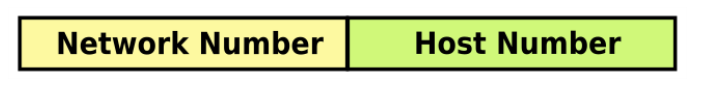
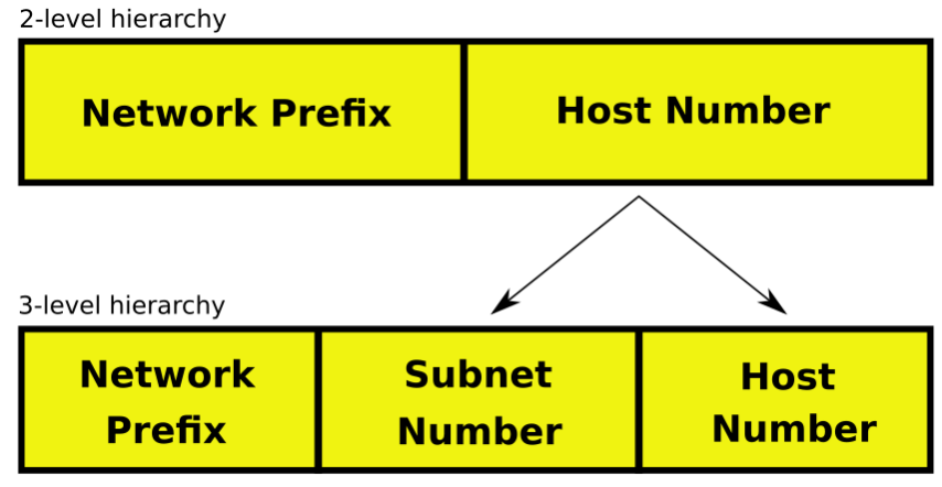
The initial way of grouping the 32 bits was called “2-level addressing
hierarchy”. In that terminology, the 32 bits of the address are split in
two groups, of 16 bits each, called the “Network Number” and the “Host
Number” as seen in the following picture:
A while after the 2-level addressing was introduced, a new way of
representing the addresses started to become more popular, because
allowed a greater flexibility over the simple splitting of the address
in two groups of 16 bits each. The Classful IP address format was born.
A different amount of bits now represented the Network number, or
network prefix, the number of bits depending on the class of the IP
address. Class A, Class B, and Class C where introduced. Each class
fixed the boundary between the network number and the host number.
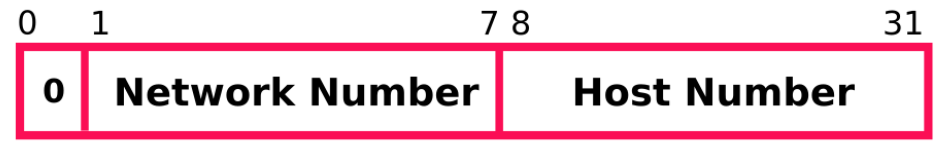
With Class A, the most significant bit is set to 0 and the next 7 bits
are actually used for the Network Number. As a result, the Host Number
is made up of 24 bits. There can be only 27 - 1 = 127 Class A networks
in the whole Internet, each with up to 224 -2 = 16,777,214 host numbers.
Two host numbers are lost to account for the address 0.0.0.0, which
represents the default route, and the address 127.0.0.0, which
represents the address of the loopback function, used mostly to test the
local connection of a device, or for internal communications within the
device itself.
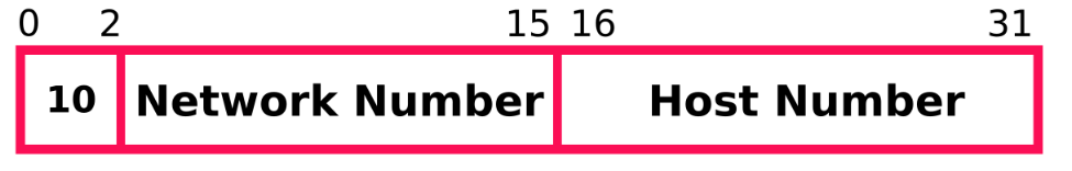
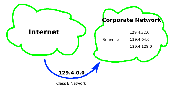
With Class B, the first two bits are set to '10' and the next 14 bits
are used for the Network Number, resulting in up to 214 = 16384 Network
Numbers, each with up to 65,534 host numbers per network.
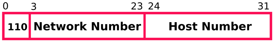
With Class C, the first 3 bits are set to '110' and the following 21
bits are used for the network number, resulting in up to 2,097,152
Network Numbers, each with only 254 host numbers.
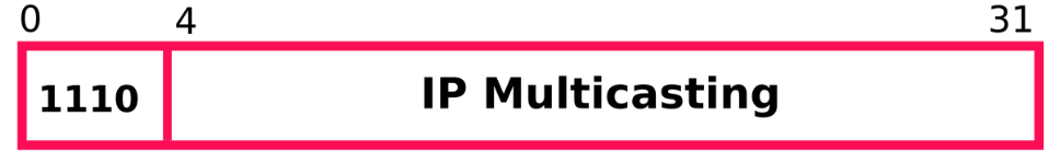
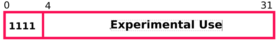
There are actually 2 more classes, called D and E. However, these last
two classes are used only for special purposes.
Class D is used for IP multicasting, a way to address several hosts at
the same time. The first 4 bits of the address are set to '1110' and the
remaining bits are the multicast address.
Class E is for experimental use. The address begins with the four digits
'1111' and the remaining are those for experimental usage.
Another way of grouping the bits of the IPv4 standard is the so called
dotted notation, more human friendly than the classful notation. In the
dotted notation, the 32 bits are all grouped in four 8 bit blocks. Each
8 bit block is represented by its decimal value. Each value is then
separated with a dot. This notation assumes the following form:
xxx.xxx.xxx.xxx
where each ‘x’ represents a decimal digit. Each group becomes therefore
a number between 0 and 255. Here are some examples:
192.168.1.57
126.35.12.4
180.254.168.111
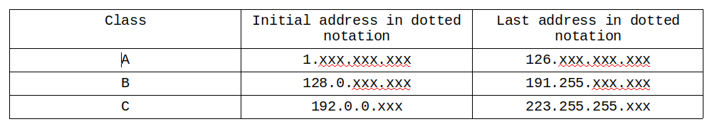
If we want to compare the classful notation with the dotted notation, we
can see the following:
In the above table, the xxx groups identify the Host Number in the IP
address.
At some point after the standard IPv4 was created, network engineers
started seeing the limitations of the classful notation, so changes were
made to the standard to introduce what was called “subnetting” (circa
1985). The concept is simple: instead of dividing the whole internet in
a limited amount of classes, they thought of dividing the whole
addressing space into subnetworks, or subnets. And each subnet could be
further divided into smaller subnets, and so on and so on.
Each subnet is identified by the number of bits that identify its index,
thus going to the concept of Network Prefix instead of Network Number.
Service  providers could assign subnets instead of classes to
individuals and companies. Each of them could still create their own
internal hierarchical structure splitting the given subnet in further
subnets.
Since the number of bits that identify a subnet was now variable, the
need arose to be able to identify how many of the 32 bit addressing
where identifying the subnet and which bits where identifying the host
numbers.
It was decided to introduce the concept of masking. Each subnet space is
therefore accompanied by a set of 32 bits that specify which are the
network prefix bits and which are the host number bits. For example:
192.168.1.0/255.255.255.0
In the above address, the numbers on the left of the / symbol identify
the first address of the subnet; the numbers on the right side identify
the mask. Each decimal number on the mask can be represented by its
corresponding binary form. In essence, the mask is made of a number of
‘1’ followed by a number of ‘0’. The ‘1’ represent the digits in the
network prefix, the ‘0’ represent the digits in the host number.
In the above example, there are 24 ‘1’ in the mask, therefore
identifying the first 24 bits of the full IP address as the network
prefix. The remaining digits in the mask are 8 ‘0’, which identify the 8
bits of the host number. Therefore, this is a network that has prefix
192.168.1 and has up to 256 host numbers. In other words, the IP
addresses that belong to this subnet are all those in the following
range:
192.168.1.0 - 192.168.1.255
Another notation for the same mask is the following:

192.168.1.0/24
The “/24” identifies the number of bits that provide the network prefix,
which is 24, in this example. It is called the prefix length.
Basically, the original host number is split in two parts, the subnet
number and the actual host number.
This technique allows for a better distribution of the IP addresses on
the Internet. Furthermore, subnets can be defined entirely within the
boundary of an organization network. Routers within that organization
take care of resolving the addresses to reach each host. The Internet
routers do not need to know the details of the subnets and, therefore,
the corresponding routing tables are simplified.
More in general, there are three main advantages in using subnetting:
1) global internet routing tables don't grow when new subnets within a
private organization are added.
2) Local administrators can create new subnets within the organization,
without the need to obtain a new network number from the Internet.
3) Route flapping (the rapid changes on routes in the subnets) does not
affect internet routing tables.
Private network routers use subnet masks to identify their subnets. As
in the Internet masks, bits in the subnet mask are set to ‘1’ if they
are part of the extended network prefix, they are set to ‘0’ if they are
part of the host number range.
When designing subnet partitioning within an organization, 3 rules have
to be verified, so that the correct network index can be requested:
1) how many subnets are currently needed for the organization?
2) how many subnets will be needed in the future for the organization?
3) what is the max number of hosts required within each subnet in the
future?
Another way of subnetting is to have a single IP address assigned by the
Internet provider and use private subnetting in the organization
network. Routers in the organization network are equipped with a service
named NAT, or Network Address Translator. NAT translates the internal IP
addresses in the organization to the one external IP address and vice
versa. This method totally hides the configuration of the organization
network to the external world, adding as a bonus an increase in
security.
Many are familiar with this setup, because it is what a service provider
does when assigning an IP address to a household. Although there is a
single IP address to commnicate with the Internet, each device within
the household has its own IP address in the Private Network.
IP addresses available to build Private Networks must be in one of the
following ranges:
10.0.0.0 – 10.255.255.255 (/8 mask)
172.16.0.0 – 172.31.255.255 (/12 mask)
192.168.0.0 – 192.168.255.255 (/16 mask)
These ranges are all reusable. It means that different private network
may use the same IP address ranges, because these addresses are hidden
to the external world through the NAT service.
It is also worth noting that back in 1993 the Internet was quickly
running out of available IP addresses. The IETF (Internet Engineering
Task Force) then came up with a way to better use what was left of the
IP addresses. That idea worked so well that, as of today, we can still
use IP addresses that were saved using that idea.
What the IETF did was to create the concept of Classless Inter-Domain
Routing, or CIDR for short.
With that innovation, each Network prefix could be provided with any
number of digits, using a mask to identify their number. This technique
allowed to better split the IP addresses in different networks for
different organizations, thus saving a number of IP addresses that
otherwise would have been wasted. IPv4 routing would not work anymore
since a long time, if it wasn’t for this clever and simple idea.
But, regardless of the clever techniques used to save on the number of
wasted IP addresses, IPv4 addressing space has less and less available
IP addresses available to build new networks.
Introducing IPv6, the solution to the exhaustion of IP addresses on the
Internet.
IPv6 is an address made of 128 bits, instead of the 32 of IPv4.
Therefore, the max number of available addresses is 2128 =
340,282,366,920,938,463,463,374,607,431,768,211,456. That is over 340
billions of billions of billions of billions of addresses. It is now
believed that this number of IP addresses will last forever, but will
it?
Let’s see how IPv6 works.
There are three ways to represent an address in IPv6 format. These are
different than the IPv4 notation, because it needs to account for so
many bits. In fact, we still group the bits in blocks, but now these
blocks are 8 instead of 4 and are made up of 4 hexadecimal digits
instead of 3 decimal digits. The first of the 3 notations is the so
called “full notation”, which is structured as follows:
xxxx:xxxx:xxxx:xxxx:xxxx:xxxx:xxxx:xxxx
Here is an example:
fd00:04e8:aac5:459b:1234:abcd:ffff:01f5
The second notation, called “compressed notation”, allows to save space
when 1 or more consecutive blocks are made of all zeros. In that case,
we replace all the consecutive blocks with ‘::’. Note that this can be
done only once in the whole IP address, otherwise it would not be
possible to identify which ones are the 0 blocks.
Here is an example:
fd00::48ab:f000:017b
which is the short version of:
fd00:0000:0000:0000:0000:48ab:f000:017b
The third notation, called “mixed notation”, has been introduced for
compatibility and interworking with the IPv4 standard. The notation uses
one of the above two formats for the first 6 blocks, then it uses the
old IPv4 notation for the last 2 blocks, which comprise the last 32 bits
of the address. This way, IPv6 can handle old IPv4 addresses by
incorporating them in the new format as the last 32 bits. Note that this
is kind of equivalent in saying that now we have a massive amounts of
subnets, each equal to the size of the whole Internet addressing when
IPv4 was the only standard available.
Here is the example for the mixed notation:
1234:5678:9abc:def0:0fed:8765:192.168.1.124
IPv6 still uses masks, with the exact same meaning of IPv4. However, the
only possible notation for the mask is the slash format.
Example: xxxx:xxxx:xxxx:xxxx:0000:0000:0000:0000/64
It would be really cumbersome having to type 8 blocks of 1 and 0 for a
mask, otherwise.
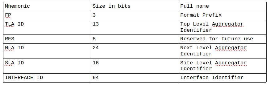
It is worth noting that, in IPv6, the Network Prefix is actually split
in 5 separate fields, used to aggregate the most significant bits in a
way that is easier for the routers to analyze the addresses and
determine the correct routing to apply to packets. Although this is not
the place to be so detailed, here is the list of the names of these
fields and their size:
Note that the table also reports one extra field, the Interface ID,
which corresponds to the Host ID in the IPv4 notation. However, the
Interface ID is actually the ID of an interface on the host. If the host
has multiple interfaces, it can have multiple Interface IDs, or IP
addresses.
Finally, IPv6 has the ability to provide extra level of functionality
and, in particular, security, with respect to IPv4:
Streamlined IPv6 header
Stateless and Stateful Configuration
Built-In security (Ipsec)
Better support for Quality of Service (QoS)
Real time performance
As IPv4, also IPv6 has a number private network defined in the standard.
Well, it is actually only one:
fd00::/8
This private network has the capability to identify addresses in the
subnet with 64 bits. Thus, the max number of hosts in a private subnet
are:
216 = 18,446,744,073,709,551,616
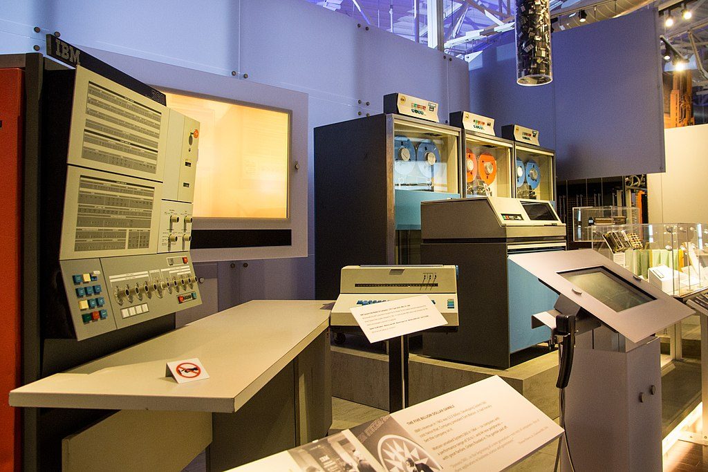
My very first computer was a mainframe IBM 360. Well, it wasn’t mine, nobody owned a computer back in the seventies. The 360 was the mainframe available at the university where I studied Electronics Engineering, the University of Palermo, in Italy. It ran under an operating system that was called DOS, an acronym for Disk Operating System.
IBM System-360 Model 30 at Computer History Museum, Mountain View
At that time, personal computers did not exist yet, so I learned how to program by using piles of punch cards. It wasn’t until the eighties that I was able to put my hands on a much smaller scale computer, capable of interactions through a video screen. Those were the times of the Commodore computers, the first Apple, and the Sinclair.
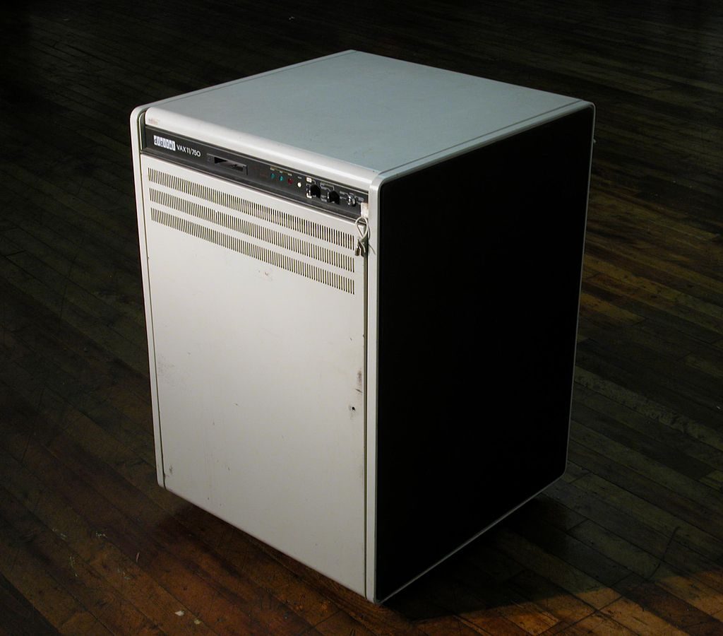
In the mean time I started working for a big telecommunication company, so I started also putting my hands on minicomputers, like the VAX 750. The OS of choice, at the time, was VMS first (Virtual Memory System), and then UNIX (Uniplexed Information and Computing Service). UNIX was a great Operating System, with an innovative way of seeing all the devices connected to it (everything is a file in UNIX). Using UNIX for all my needs as a programmer for telecommunication systems was really fun and easy and I kept growing fond of it day by day.
Attribution: Retro-Computing Society of Rhode Island [CC BY-SA 3.0 (https://creativecommons.org/licenses/by-sa/3.0)]
VAX-11-750
And, finally, the IBM personal computer arrived and, with that, MS-DOS.
MS-DOS was an OS similar to UNIX, in certain ways, but much more limited in capabilities and cumbersome to use to type commands. Having the habit of using UNIX, MS-DOS wasn’t exactly my ideal of Operating System.
Attribution: Vintageibmmt [Public domain]
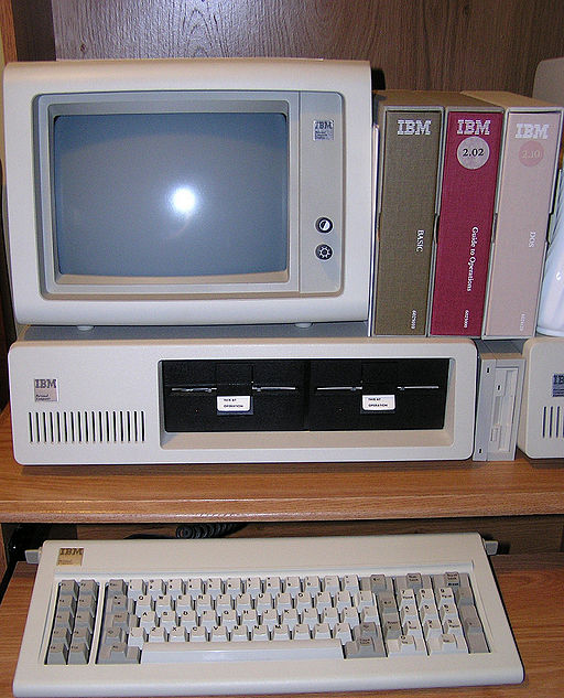
IBM 5150 PC
Finally the first graphical interfaces started to appear. They were actual programs running on top of UNIX and they were very efficient and easy to use.
And then, the first graphical interfaces started appearing also on Apple and IBM PCs. That was the time when the first IBM PC compatible computer entered my home. It was equipped with MS-DOS 5.0 and Windows 3.0.
With that PC, I learned how to make programs with graphical interfaces and the world of personal computing suddenly became much more interesting.
Also my work improved in that period of time. I moved to the USA and worked for a while for the AT&T Bell Labs. Later, AT&T Bell Labs let go its developmet branch and Lucent Technologies was born. There I soon started working on a new telecom system named Softswitch. Softswitch was heavily based on a new Operanting System called Linux, that looked practically identical to UNIX, at least from the high level point of view. I learned that Linux could be easily and freely installed on a PC and so, one day, I took an old machine that I had around at home, downloaded Fedora Core 8, and installed it on that old PC.
I was really amazed when I found that Fedora was able to run really fast on that old system, and that had so many choices of graphical interfaces, many resembling those that I was used to in the UNIX environment. I also discovered that Fedora repositories were full of free applications, many of them a perfect replacement of those applications I daily used in the Windows environment.
So, one day, I decided to switch from MS Windows to the Linux distro Fedora and see if I could use it for day to day tasks at home without relying on Windows apps anymore. It was a success and, within a few months, I completely abandoned Windows in favor of Fedora-Linux, never to return anymore to Microsoft and its heavy to run applications that needed newer and more powerful machines every year. The one and only application that I wasn’t able to replace was the one to prepare my tax returns. But for that, I just used a virtual machine under Linux running Windows in it. For anything else, I used the Fedora distro of Linux.
Thank you Linus Torvalds for having created such a viable Operating System!
Today I use Linux for everything (besides the tax prep app). I use it for programming personal applications, to handle the family budget, to play games, to handle my multimedia collection of videos, music and pictures. I also use it to create my video contents that I periodically publish on YouTube under the brand eleneasy (I also have a companion site eleneasy.com, where I expand on the subjects I present on YouTube).
From time to time I also like to experiment with different Linux distros. I tried CentOS, Debian, Ubuntu and several others. However, no one operating system has ever been able to provide me with what Fedora makes available. I like the cutting edge feel of Fedora: every time something new happens in the world of Linux, Fedora is always the first place where you see it happen.
But, there is always a but…
Over time, the computer at home became for me more and more a tool to use, not a programming environment like the one I use at work. And because of that I started having doubts about the cutting edge thing. In fact, from time to time, I found myself spending some time to fix things that stopped working, or at least stopped working the way they did before. So, I started thinking to use a different distro that would give me more stability, more consistency over time. And so one day I decided to move to Ubuntu, which provide a Long Term Support, or LTS, kind of release, which is basically upgraded only to fix bugs, but remains in general constant for a few years.
I took the decision to move to Ubuntu LTS when the current release was about to be replaced with a new one in a one year time frame. But I thought: what the heck, I will install the current one and upgrade to the next once it comes out, and then I will be done with upgrades for another 4 years.
What a mistake that was.
When I upgraded Ubuntu to the new LTS release, a lot of things started happening. Several programs refused to work in the new Release, others disappeared. And some of them where those I relied upon to do my work with 3D printing, blogs, electronics design, and video making.
I tried to resist for a while, working hard to make those programs work again. For some I succeeded, but for others I had to admit that they might have not worked anymore unless, probably, I reinstalled Ubuntu from scratch.
What a delusion!!!
And so, since my last resort was to reinstall, I decided to go back to Fedora, currently on version 29. As soon as I did that, I regained control of all those programs I had lost and, for some of them, I also gained some new features and a much needed higher execution speed. I promised myself that I will never again move away from Fedora. Little glitches on every new release are, at the end, easy to fix and live with. But the bad Ubuntu experience… never again.
I have to say that the choice of using Ubuntu was not an easy one. When I did that, I tested several distros to see how they behaved with the applications I needed to use the most. Ubuntu was the definitive winner and, probably, if I wasn’t the power user I am, Ubuntu would have been just fine for me. But, in my terms, I like and need continuous innovation that doesn’t break. Little glitches I can handle. And so my best option remains Fedora.
Not to say that Ubuntu is a bad distro. Not at all. Ubuntu works just fine for normal users, those that do not have a good understanding of what happens behind the scenes of an OS and so are happy to use a system that takes away all the burdens of acting as a system administrator more often than they would like. Ubuntu is perfect for the simplified way of installing it, for the automation in software updates, and a lot of other things.
However, Fedora is the best solution for my needs. I like the cutting edge side of the distro, providing always the latest capabilities (that sometimes need a little tweaking to make them work the way you want). After all, Fedora is just that, a trampoline platform for testing new technology that later is incorporated in the Red Hat distro, which is basically the commercial edition of Fedora, kind of equivalent to the LTS for Ubuntu.
But Fedora works for me as is, and I made the promise to myself to never cheating her again for another distro somewhat less capable of her.
And you? What Operating System runs on your personal computer, being it a desktop or a laptop, or whatever else? I’d like to make a little poll about it to see what kind of OS is used by my followers. Please drop me a small comment, maybe with just the name of the OS you use, if you don’t want to spend much time. It could help me for better aiming future posts on this site. I suspect the most people uses Windows, followed by OSX and Linux. And then there are the Chromebooks, and FreeBSD, and several others. Which one is yours?
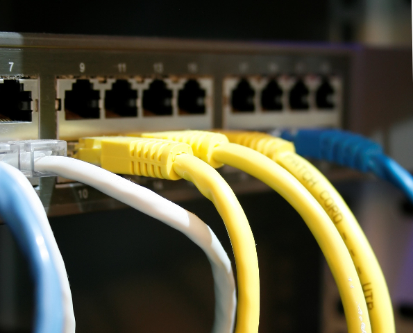
Bandwidth and Throughput! There is a lot of confusion about these terms, what they mean, what you should care for.
Let’s try some definition first, and then let’s go into the details.
From the electrical perspective, Bandwidth is the max amount of frequency a cable can support without signal degradation. In the networking field, this is usually confused with the Max Data Rate that a link can support, either physical (i.e. a cable) or wireless (i.e. WiFi).
In reality, Bandwidth and Max Data Rate are not the same thing. The Max Data Rate that a link can support depends on the Bandwidth, but also depends on the carrier modulation supported by the link (please take it as it is, this is not the place to start a digression on telecommunications theory, but if you really want to know, please drop me a comment and I will post an article just for that).
Also, the difference between the bandwidth and the max data rate depends on the protocol being used and, if more than one protocol are stacked together (see my post on the OSI model), you have different max data rate values for each of the protocol layers. The higher is the protocol layer, the lower is the max data rate.
Bandwidth is measured in Hz (hertz) and its multiples (kHz, MHz, GHz).
Data Rate is measured in the number of bits sent in one second, or b/s and its multiples (kb/s, Mb/s, Gb/s). Note that I mentioned bits, not bytes. Carries sell or rent their data links using b/s as measurement unit.
Since a byte is made up of 8 bits, 1 byte/s = 8 b/s. “byte/s” is usually abbreviated as B/s.
So, when a carrier sells you a data link capable of transporting 10 Mb/s, in reality that link can transport only 10/8 = 1.25 MB/s. Keep that in mind, when you do your calculations to figure out how much do you need to buy.
Also, the carrier will most probably tell you that it is selling or renting you a data link with a bandwidth of 10 Mb/s. But, remember, that is not really bandwidth, it is instead maximum data rate.
The real data rate that the link will be able to carry will be definitively less than that “bandwidth” they are selling you. In fact, that data rate is what is called throughput. In these correct terms, what they sell you as bandwidth is in reality called the maximum throughput that the link can support.
The real throughput will always be less than the max throughput for several reasons. Among others:
latency (delay in transmitting/receiving a data packet)
computational capability of the network elements between the sender and the receiver of the data packets. The throughput will never be greater than the smaller throughput encountered in the network elements in the path.
amount of users using the same link, which will cause a contention in the usage of the link itself
type of protocol, because each protocol uses different header sizes to envelop the packets it is sending/receiving, and the bytes in those headers add up to the bytes of actual data being transmitted/received
Let’s dig a little bit more in these 4 bullets, and remember that there are several more reasons why the real throughput is smaller than the max throughput.
In order to do so, let’s compare a data link with a pipe transporting water.
The max throughput, which many call improperly bandwidth, is the amount of water that the pipe can transport, given its physical size, the diameter of the pipe, in particular.
You can easily figure out on your own that the max amount of water the pipe can carry is not necessarily what the pipe will carry at any given time. Think of the case where you are providing water through a valve that can regulate the amount of water through it. If the valve is closed, there will be no water in the pipe. If the valve is half open, there will be an amount of water flowing in the pipe, and the rest of the pipe will be filled with air.
That said, let’s see what the latency causes in a data link, compared with the pipe and the water. Most protocols, when sending a data packet, will wait for a response from the other end that confirms the reception of the packet before sending the next one. Since it takes a certain amount of time for the sent packet to reach the far end and then for the response to come back (this is the latency, or delay), the data link will not be used to transmit data for that hole interval after a packet is sent. This is the equivalent of opening the valve of the water for a short amount of time, then close it. Then we wait for the water to reach the other end of the pipe and then we wait some more time for somebody else at that end of the pipe to tell us that the water is arrived. Only then we open the valve for another short moment. You can see that the pipe will remain empty for most of the time, and that is what happens with a data link, because of the latency.
The computational capability of the network elements can be assimilated to the size of the pipe along the way. If the pipe becomes narrower in certain parts of the path, the whole pipe will be limited in the amount of water that can transport at any given time by the smaller of all the pipe diameters along the way.
Amount of users using the data link. The more users the less throughput. Think at the number of users as the number of valves that input the water into the pipe. With two users, if one pushes an amount of water equal to half the amount the pipe can transport, the other user will be at most able to push half the amount of water in to the pipe, because that way the pipe will be totally filled, between the two user. Now, think about if one user opens almost completely the valve, and therefore uses most of the capacity of the pipe. Even if the other user opens the valve in the same amount, just because he did it a little later that the first user, it won’t be able to push the amount of water he wants.
For the effect due to the type of protocol, think it this way: each protocol introduces an overhead in terms of extra bytes to provide certain information that depend on how the protocol works. So, you have your data, then you have to send them in a packet. The number of bytes you send is equal to the number of bytes of your data plus the number of bytes of the overhead introduced by the protocol. In addition to that, when you think that normally you will use a number of protocols stacked to each other, and considering that each protocol sees the data packet built by its predecessor in the stack as pure data and, therefore, adds its own overhead, you see that you may end up with the case where the most bytes you send are due to the involved protocols and just a few are the actual data you wanted to send. So, although you are filling the pipe with all this data, only a percentage of it is what you meant to send in the first place.
Each of the above problems has its own solution to minimize the impact to the real throughput. However, keep in mind that there is only so much you can do, and there is no way you can address all the possible causes of throughput reduction. So, at the end, the final throughput you obtain in your data link will never be that close to the max throughput. I can actually tell you that, in most of the cases, you are very lucky if you can reach 30% of the max throughput, unless you are using the link in some special way (but this is a whole different story).
All in all, when you design your network, keep in mind that in order to use as much throughput as you can, you have to make sure that the links you are using are at least 3 times oversized with respect of what you need. But, in addition to that, you have to make sure that all the network elements (routers, DNS servers, and so forth), are built to withstand a throughput higher than the one you need.
For example, let’s say you have links at 100Mb/s. And now you have a router that can connect to 100Mb/s links. Also, you are in need to have a throughput across the network of at least 30 Mb/s. Then if the router from above connects to 10 of those links, and each link needs to transfer at least 30 Mb/s of data, then your router has to have a total throughput of at least 10 x 30 = 300Mb/s, even though it is connected to 100Mb/s links. If your router is not capable of doing that, you will never be able to use your links at the best of their capabilities.
Now, think at what kind of throughput a wireless router or access point needs to have if it needs to support just the 802.11g protocol, which has a max throughput of 54 Mb/s, and the number of users is 20. The throughput of this network element should be 54 x 20 = 1080 Mb/s ~= 1 Gb/s !!!
Interesting, isn’t it?
Maybe now you understand why your wireless network is not capable of supporting the amount of users that attach to it, and why everything slows down to a crawl when several users are connected, while everything is perfectly fine if only one or two users are using the WiFi connection.
INFORMATION IN THIS WEB SITE IS PROVIDED "AS IS" WITHOUT WARRANTY OF ANY KIND, EITHER EXPRESS OR IMPLIED. THE USER ASSUMES THE ENTIRE RISK AS TO THE ACCURACY AND THE USE OF THIS INFORMATION.
Trademarks: All brand names and product names used in this web site are trade names, service marks, trademarks, or registered trademarks of their respective owners. Dazzling Solutions is not associated with any product or vendor mentioned in the site, unless otherwise specified.